Moodifier: MLLM-Enhanced Emotion-Driven Image Editing

3. Methodology

3.1 MoodifyCLIP

Although our human validation study confirms the decent quality of LLaVA-generated captions, we acknowledge that hallucinations are inevitable at this scale. However, the fine-grained emotional context these rich descriptions provide is invaluable, capturing nuances that shorter captions cannot. To handle longer descriptions, we adopt a positional embedding interpolation strategy. To balance accuracy and detail, MoodifyCLIP incorporates:

Global Contrastive Loss (GL)

We adopt CLIP's visual encoder E_i and text encoder E_t to map inputs into a unified embedding space: I^f = E_i(I), T^f = E_t(T^f). While detailed captions capture specific emotional triggers and nuanced affective dimensions missing from existing datasets, concise summary captions remain crucial for holistic image comprehension. To balance granular details with global understanding, we add T^s = E_t(T^s). Note that T^f contains the complete five-sentence caption from our LLaVA annotations, while T^s only includes the first and last sentences (i.e., summary caption and emotion assessment).

We obtain the text-to-vision loss via InfoNCE contrastive learning between visual representations I^f and textual embeddings T^f as: L_f = (L_f^t2v + L_f^v2t)/2 with explicit formulation:

L_f^t2v = −∑_i=1^N log exp(cos(I^f_i, T^f_i)/τ) ∑_j=1^N exp(cos(I^f_j, T^f_i)/τ)

L_f^v2t = −∑_i=1^N log exp(cos(T^f_i, I^f_i)/τ) ∑_j=1^N exp(cos(T^f_j, I^f_i)/τ)

Equation 1: Global Contrastive Loss

Similarly, we add an objective for the global summary caption and emotion assessment: L_s = (L_s^t2v + L_s^v2t)/2.

Fine-grained Loss (FG)

Next, to fully utilize our hierarchical annotations, where each emotional stimulus prompt is carefully engineered to describe distinct affective elements, we align each with its corresponding regions of interest within the image. We first compute cross-attention weights between fine-grained text embeddings (T^fg) and image patch embeddings (I^fg), yielding a similarity matrix W = {w_i,j}. Applying these weights ensures that each emotional stimulus description is primarily focused on its relevant visual regions while differentiating itself from others.

The attention-weighted visual representation for each stimulus j is computed as:

I^fg_j = ∑_m=1^M w_i,j ∑_j³ w_i,j I^fg_m

Equation 2: Attention-weighted Visual Representation

We implement a contrastive objective for such region visual representations as:

L_fg^t2v = −∑_i=1^N ∑_j=1³ log exp(cos(I^fg_i,j, T^fg_i,j)/τ) ∑_m=1^M exp(cos(I^fg_i,m, T^fg_i,j)/τ)

L_fg^v2t = −∑_i=1^N ∑_j=1³ log exp(cos(T^fg_i,j, I^fg_i,j)/τ) ∑_m=1^M exp(cos(T^fg_i,j, I^fg_i,m)/τ)

Equation 3: Fine-grained Alignment Loss

Symmetrically we get L_fg = (L_fg^t2v + L_fg^v2t)/2. This fine-grained alignment mechanism helps develop a sophisticated understanding of which visual elements trigger specific emotional responses.

Fine-grained Loss Visualization — **Figure 3:** Illustration of how MoodifyCLIP processes both global captions and localized emotion triggers to create fine-grained alignments between text and image regions.

Optimal Transport Loss (OT)

Now that we have the fine-grained loss for specific connections (zoom-in), such as matching a smiling face region with text about happiness or tearful eyes with sadness, we take a bigger-picture (zoom-out) via optimal transport. Mathematically, it solves the matching problem by finding the most efficient overall assignment between all image regions and all text descriptions while respecting their similarity as in the matrix S = ⟨I_fg, T_fg⟩_batch, which translates into transportation costs (distance matrix) as: W = 1 − S.

Then, by asking the question, "What's the most efficient way to match all the emotional elements in these images with all the emotional concepts in these texts?", we use the Sinkhorn algorithm to find the optimal global assignment while respecting local emotional nuances:

T_ot = sinkhorn(W)

= arg min_P∈Π(a,b) ⟨W, P⟩ − ϵH(P)

where a and b are uniform distributions over image regions and text features respectively

Equation 4: Optimal Transport Formulation

where a and b are uniform distributions over image regions and text features respectively, while Π(a, b) is the set of all possible transport plans with these marginals, and H(P) is an entropy regularization term.

Here higher values in T represent preferred transport paths (where it's "cheaper" to move mass), hence amplifying signals from high-similarity pairs while downplaying mismatches. This is particularly valuable for emotions, which are often ambiguous and overlapping. The final OT loss is computed as L_ot = CrossEntropy(T_ot⊙S, I), where I is the identity matrix.

Our total loss combines all components as:

FINAL LOSS

L_moodifyclip = λ_f · L_f + λ_s · L_s + λ_fg · L_fg + λ_ot · L_ot

λ_f: Global weight λ_s: Summary weight λ_fg: Fine-grained weight λ_ot: OT weight

Equation 5: Total MoodifyCLIP Loss

Algorithm 1: PyTorch-like pseudocode for MoodifyCLIP

# I_b, T_b, w_I, zI = minibatch of aligned images
# T[b, i]      = minibatch of aligned texts
# T_summary[b, i] = minibatch of summary captions
# image_encoder = Vision Transformer (ViT)
# text_encoder  = Text Transformer (BERT)
# d_I          = dimension of image features
# d_T          = dimension of text features
# M            = number of image patches/tokens in ViT
# N            = number of sentences in emotional annotations [=5]
# f/g          = suffix for global features and losses
# s            = suffix for summary features and losses
# fg           = suffix for fine-grained features and losses
# ot           = suffix for optimal transport components
# w_g, w_s, w_fg, w_ot = weights for different components

# Extract features from images and text
I_g = image_encoder(I)  # [b, d_I]
T_g = text_encoder(T)  # [b, d_T]
T_s = text_encoder(T_summary)  # [b, d_T]
I_fg = stack(text_encoder(T) for T in T)  # [b, N, d_T]

# #### Global image-text contrastive loss
loss_g = InfoNCE_loss(I_g, T_g)

# #### Summary sentence contrastive loss
loss_s = InfoNCE_loss(I_g, T_s)

# #### Fine-grained contrastive loss
I_fg_patches = reshape(I_g, [-1, M, d_I])  # reshape to patch dimension

# Compute attention-based feature alignment
w_align_weights = einops.einsum(I_fg_patches, T_fg, 'n k p, n p d -> n k p')
I_fg_grouped = einops.einsum(w_align_weights, I_fg, 'n k p, n p d -> n k d')

# Compute loss from token-region alignment
w_flat = einops.rearrange(w_align_weights, 'n k d -> (n k) d')
I_fg_grouped_flat = einops.rearrange(I_fg_grouped, 'n k d -> (n k) d')
T_fg_flat = einops.rearrange(T_fg, 'n k d -> (n k) d')
loss_fg = InfoNCE_loss(I_fg_grouped_flat, T_fg_flat)

# #### Optimal transport loss
sim = einops.einsum(I_fg, T_fg, 'n p d, n k d -> (n p) k')
sdist = 1.0 - sim
P_ot = sinkhorn(sdist)
sim_ot = torch.sum(P_ot * sim, dim=1, 2))
loss_ot = cross_entropy(sim_ot, torch.eye(n))

# Combine losses with weights
total_loss = w_g * loss_g + w_s * loss_s + w_fg * loss_fg + w_ot * loss_ot

3.3

Moodifier

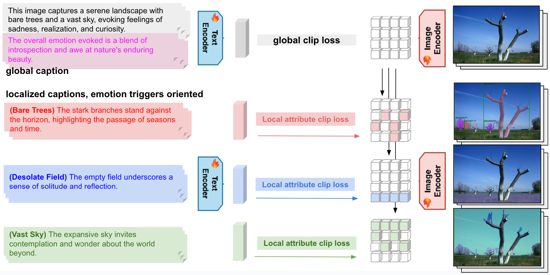
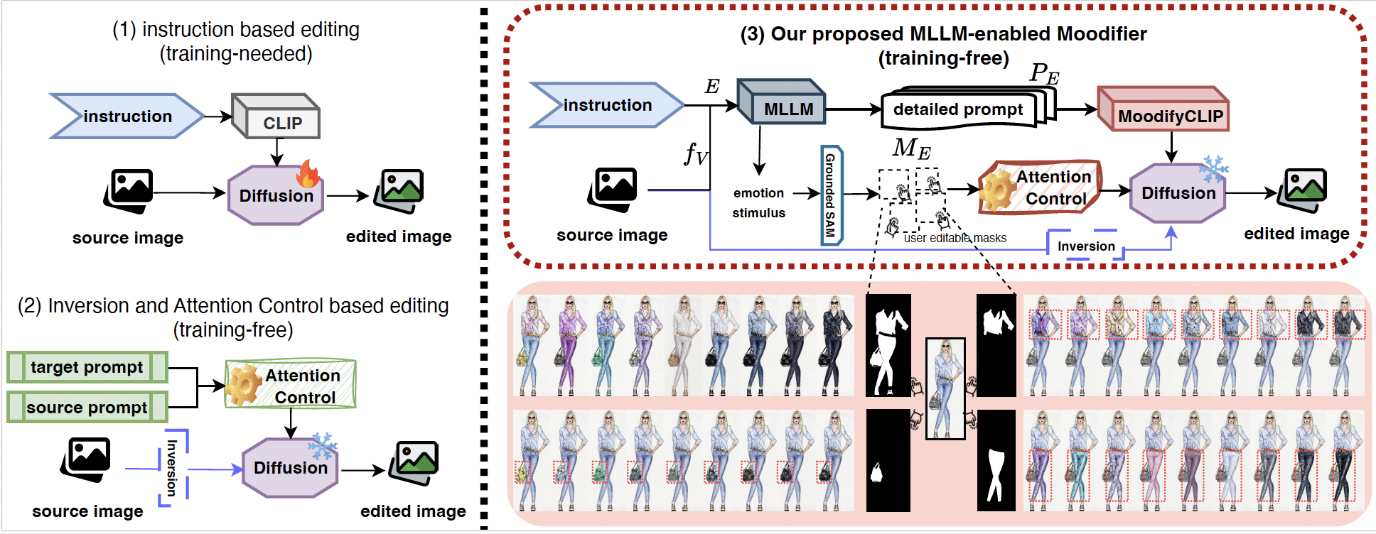
With MoodifyCLIP fine-tuned on MoodArchive, we propose Moodifier, a training-free, emotion-driven image editing system. The Moodifier workflow first extracts visual features f_V = Enc_vis(V) from the source image, enabling MLLM (in our case we applied LLaVA-NeXT) to generate emotion-specific prompts P_E = MLLM(f_V, E) and attention maps M_E that identify where modifications should occur. These outputs then guide the diffusion process to produce the emotionally transformed image.

More specifically, we adopt the non-iterative inversion approach to obtain the latent representation z. Inspired by Prompt-to-Prompt, we then manipulate the cross-attention mechanisms within the diffusion process to achieve precise emotional transformations. We operate on the key insight that cross-attention maps define the relationship between spatial image features and textual concepts.

Algorithm 1: Moodifier

MLLM-Enhanced Emotional Editing

                            Require: Source image V, target emotion E

                            Ensure: Emotionally edited image V′
                        
1:
fV ← Encvis(V)
2:
PE, ME ← MLLM(fV, E)
3:
PE ← MoodifyCLIP(PE)
4:
z ← Invdm(V)
5:
Initialize z*T ← z
6:
for t = T, T − 1, . . . , 1 do
7:
zt−1, Mt ← DM(zt, ∅, t)
8:
M*t ← DM(z*t, PE, t)
9:
M̃t ← BlendMaps(Mt, M*t, ME, t)
10:
z*t−1 ← DM(z*t, PE, t){M ← M̃t}
11:
z*t−1 ← (1 − 1ME>0) ⊙ zt−1 + 1ME>0 ⊙ z*t−1
12:
end for
13:
return z*0

In text-conditioned diffusion models, each diffusion step computes attention maps M_t through:

M_t = Softmax QK^T √d

Equation 6: Cross-attention Map Computation

where Q = ℓ_Q(φ(z_t)) represents visual feature queries, and K = ℓ_K(ψ(P)) represents textual feature keys. The cell M_i,j defines the influence of the j-th textual token on the i-th pixel. For emotional editing, we need precise control over which image regions should change and how. Our MLLM generates not only detailed prompts P_E but also spatial attention maps M_E that identify emotion-relevant regions.

As shown in Algorithm 1, DM (Diffusion Model) refers to a single step of the diffusion process that denoises the latent representation while computing cross-attention maps between visual and textual features. Specifically, DM(z_t, P_E, t) computes one denoising step from noise level t to t − 1 conditioned on prompt P, producing both the denoised latent z_t−1 and the attention maps M_t. We blend attention maps from the source image with those generated for the target emotion:

M̃_t = Refine(M_src, M_tgt, M_E) t ≥ τ_c M_tgt t < τ_c

Equation 7: Attention Map Blending

where τ_c controls attention strength. At early steps (t ≥ τ_c), refined attention is used to establish structure while preserving identity, whereas in later steps (t < τ_c), target attention maps enhance emotional details. Finally, the emotion stimulus maps M_E smoothly blend source and target latents only in regions that should express the target emotion, while preserving the rest of the image.

Moodifier Workflow — **Figure 4:** The Moodifier workflow illustrating how MLLM-generated prompts and attention maps guide the diffusion process to achieve precise emotional transformations while preserving content integrity.

By leveraging the capabilities of MoodifyCLIP and MLLMs, our Moodifier system enables precise emotional transformations while preserving structural and semantic integrity, offering a powerful tool for creative professionals to explore emotional variations in visual content without the need for extensive manual editing or additional training.

BibTeX

@article{,
  title={},
  author={},
  booktitle={},
  year={}
}